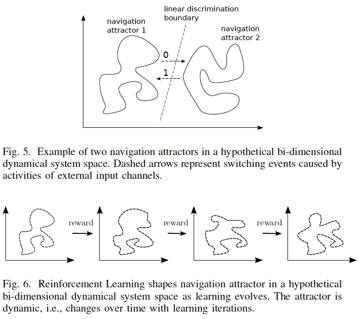
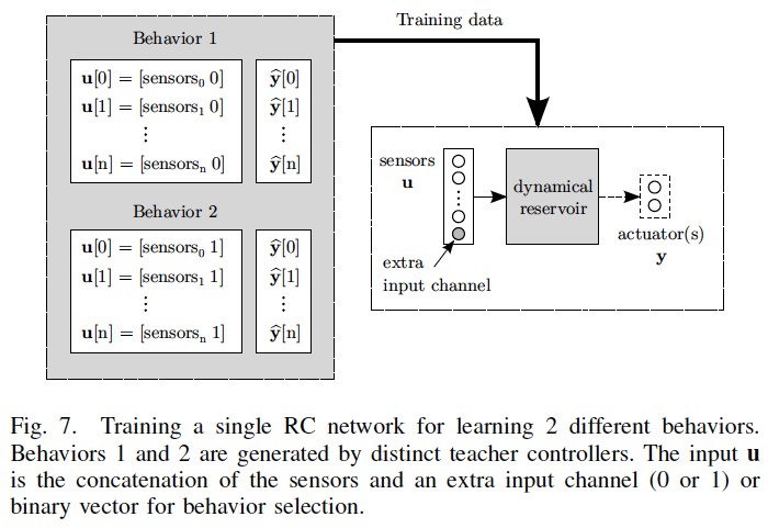
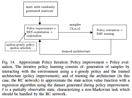
This work proposes a general Reservoir Computing (RC) learning framework which can be used to learn navigation behaviors for mobile robots in simple and complex unknown, partially observable environments. RC provides an efficient way to train recurrent neural networks by letting the recurrent part of the network (called reservoir) fixed while only a linear readout output layer is trained. The proposed RC framework builds upon the notion of navigation attractor or behavior which can be embedded in the high-dimensional space of the reservoir after learning. The learning of multiple behaviors is possible because the dynamic robot behavior, consisting of a sensory-motor sequence, can be linearly discriminated in the high-dimensional nonlinear space of the dynamic reservoir. Three learning approaches for navigation behaviors are shown in this paper. The first approach learns multiple behaviors based on examples of navigation behaviors generated by a supervisor, while the second approach learns goal-directed navigation behaviors based only on rewards. The third approach learns complex goal-directed behaviors, in a supervised way, using an hierarchical architecture whose internal predictions of contextual switches guide the sequence of basic navigation behaviors towards the goal.
During my PhD, I've worked mainly on Reservoir Computing (RC) architectures with application to modeling cognitive capabilities for mobile robots from sensor data and sometimes through interaction with the environment.
Reservoir Computing (RC) is an efficient method for trainning recurrent neural networks, which can handle spatio-temporal processing tasks, such as speech recognition. These networks are also biological plausible, as recently argued in the literature.
In my case, I used these RC networks for modeling a wide range of capabilities for mobile robots, such as:
My publications are listed and can be downloaded in Google Scholar or here.
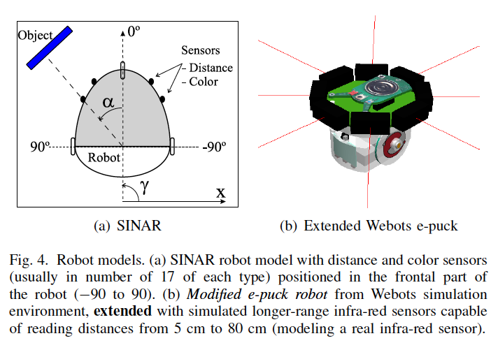
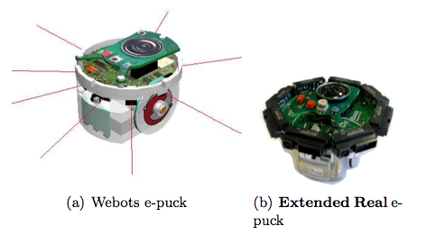
Some simulated and real robots employed in the experiments:
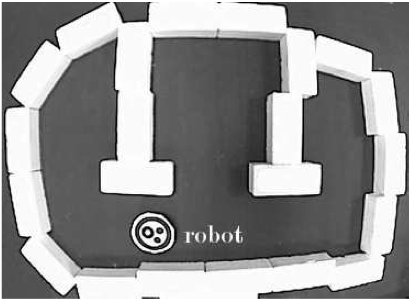
Environment used for localization experiments using the real e-puck robot:
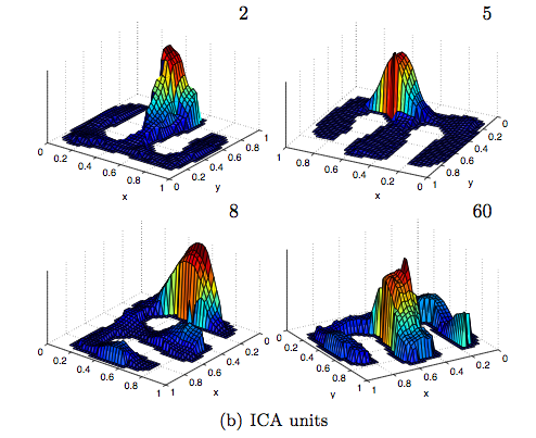
After using unsupervised learning methods for self-localization, the plots below show the mean activation of place cells as a function of the robot position in the environment.
Red denotes a high response whereas blue denotes a low response.
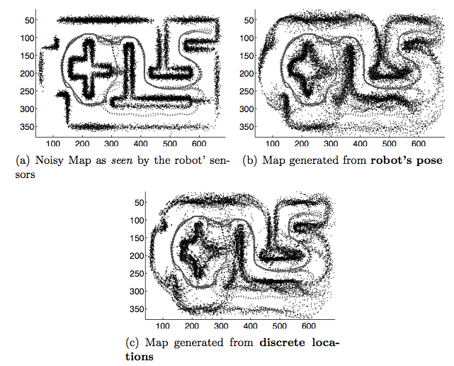
It is possible to perform map generation through sensory prediction given the robot position as input. Black points represent the sensory readings whereas gray points are the robot trajectory.
Deriving robust control policies for realistic urban navigation scenarios is not a trivial task. In an end-to-end approach, these policies must map high-dimensional images from the vehicle's cameras to low-level actions such as steering and throttle. While pure Reinforcement Learning (RL) approaches are based exclusively on rewards, Generative Adversarial Imitation Learning (GAIL) agents learn from expert demonstrations while interacting with the environment, which favors GAIL on tasks for which a reward signal is difficult to derive.
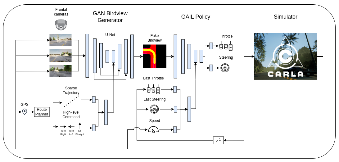
In this work, the hGAIL architecture was proposed to solve the autonomous navigation of a vehicle in an end-to-end approach, mapping sensory perceptions directly to low-level actions, while simultaneously learning mid-level input representations of the agent's environment. The proposed hGAIL consists of an hierarchical Adversarial Imitation Learning architecture composed of two main modules: the GAN (Generative Adversarial Nets) which generates the Bird's-Eye View (BEV) representation mainly from the images of three frontal cameras of the vehicle, and the GAIL which learns to control the vehicle based mainly on the BEV predictions from the GAN as input.
Our experiments have shown that GAIL exclusively from cameras (without BEV) fails to even learn the task, while hGAIL, after training, was able to autonomously navigate successfully in all intersections of the city.
Fig. 1 - Hierarchical Generative Adversarial Imitation Learning (hGAIL) for policy learning with mid-level input representation. It basically consists of chained GAN and GAIL networks, where the first one (GAN) generates BEV representation from the vehicle's three frontal cameras, sparse trajectory and high-level command, while the latter (GAIL) outputs the acceleration and steering based on the predicted BEV input (generated by GAN), the current speed and the last applied actions. Both GAN and GAIL learn simultaneously while the agent interacts to the CARLA environment. The discriminator parts of both networks are not shown for the sake of simplicity.
This research has been summarized in a paper that is under review. More details at:
Both the intermediate mid-level input BEV representation and the control policy are learned as the agent navigates in an urban town. After training, we can see the autonomous vehicle navigation in the video below:
We can also observe the learning of the Bird's-Eye view representation of the Conditional GAN embedded in the hGAIL architecture, which learns concomitantly with the GAIL policy:
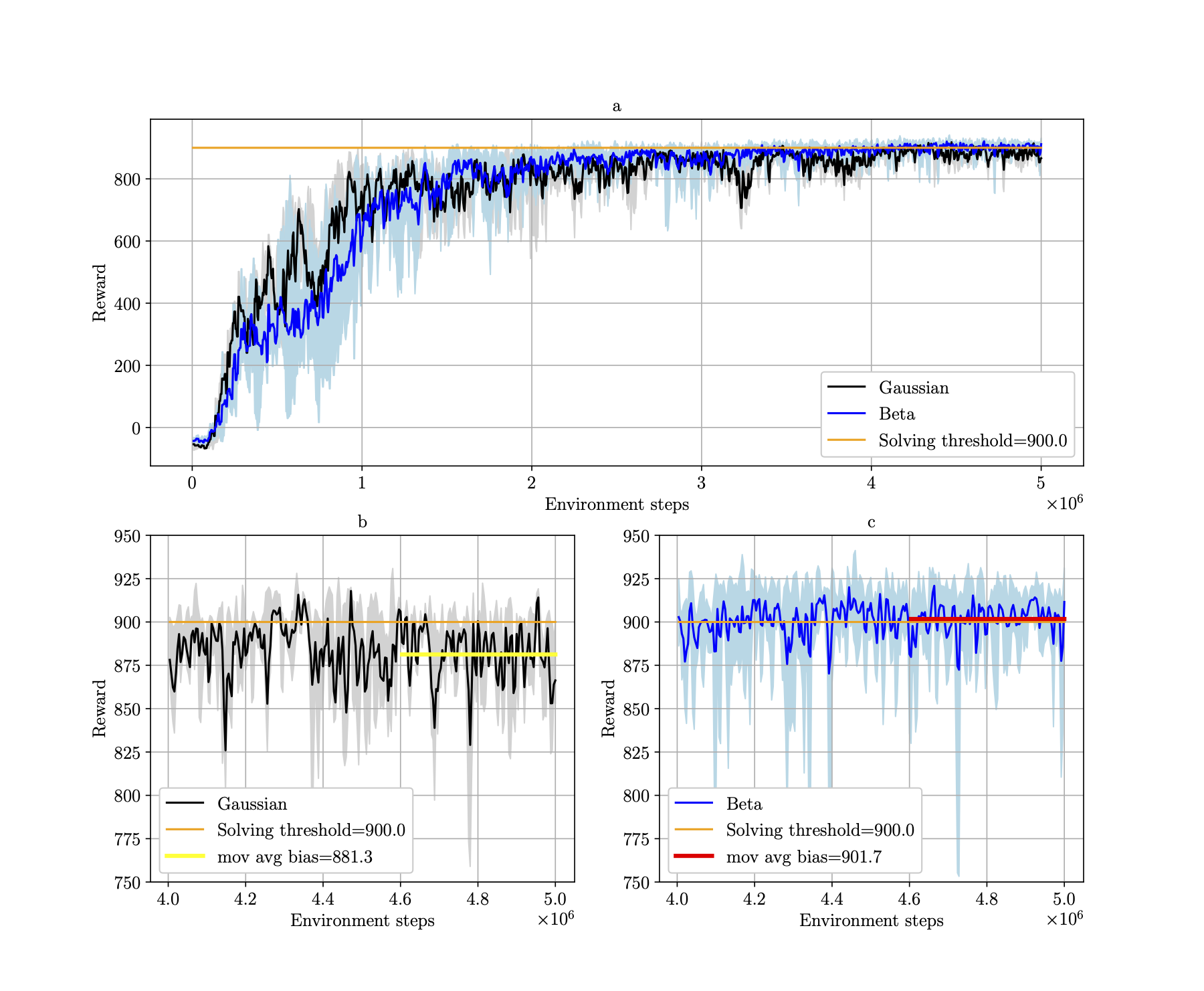
Reinforcement learning methods for continuous control tasks have evolved in recent years generating a family of policy gradient methods that rely primarily on a Gaussian distribution for modeling a stochastic policy. However, the Gaussian distribution has an infinite support, whereas real world applications usually have a bounded action space. This dissonance causes an estimation bias that can be eliminated if the Beta distribution is used for the policy instead, as it presents a finite support. In this work, we investigate how this Beta policy performs when it is trained by the Proximal Policy Optimization (PPO) algorithm on two continuous control tasks from OpenAI gym. For both tasks, the Beta policy is superior to the Gaussian policy in terms of agent's final expected reward, also showing more stability and faster convergence of the training process. For the CarRacing environment with high-dimensional image input, the agent's success rate was improved by 63% over the Gaussian policy.
The CarRacing-v0 environment simulates an autonomous driving environment in 2D.
The observation space consists of top down images of 96x96 pixels and three (RGB) color channels. The latest four image frames were stacked and given as input to the agent's network after rescaling and preprocessing them to gray scale (totalling 84x84x4 input dimensions). The action space has three dimensions: one encodes the steering angle and is bounded in the interval [-1, +1]. The other two dimensions encode throttle and brake, both bounded to [0, 1].
In the plot below, we can see the average rewards for 5 agents with different seeds for the CarRacing environment. The final performance is shown on the bottom plots at a bigger scale, for agents with Gaussian policy (bottom left) and Beta policy (bottom right).
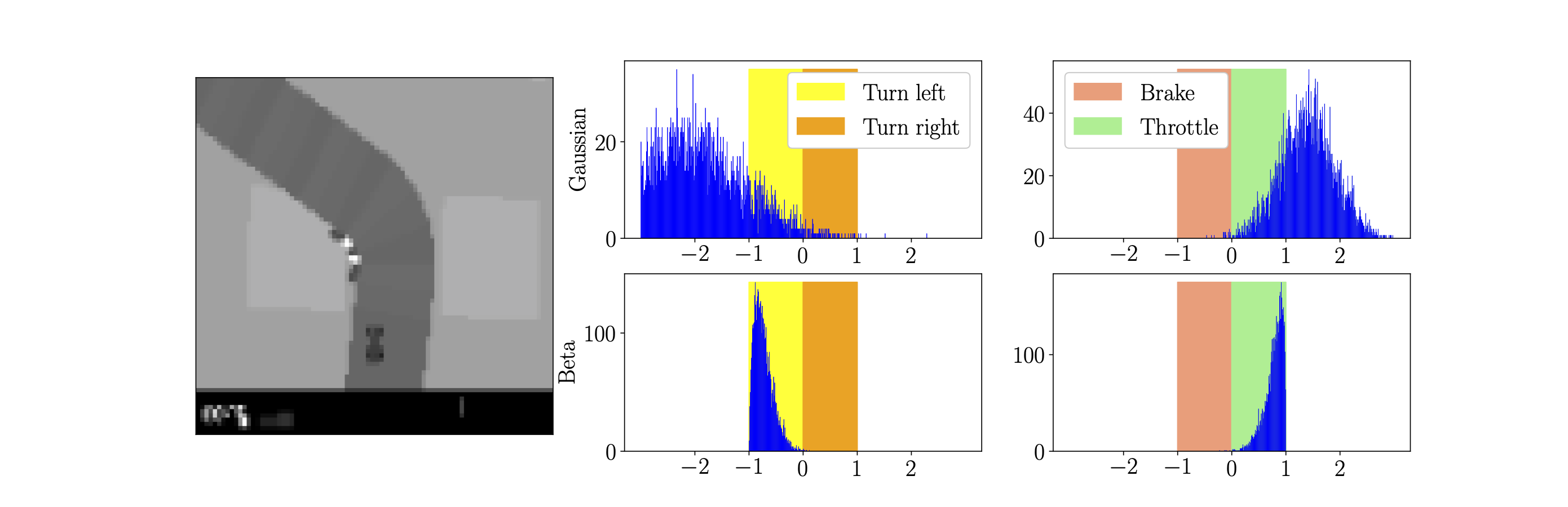
Next, we see an illustration of the Gaussian and Beta stochastic policy distributions in relation to the action space of the CarRacing environment. For a fixed observation s (preprocessed image in left plot), we sampled the Gaussian and Beta policies for 5000 actions. For the Gaussian distribution, a significant portion of the actions fall out of the valid direction and brake/throttle range (both [-1, 1]), whereas for the Beta distributions, all actions fall within boundaries.
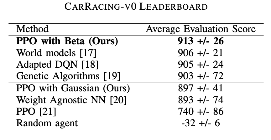
OpenAI CarRacing-v0 Leaderboard hosts a series of self-reported scores. We compare our results only to those found in peer-reviewed articles since they provide a basis for comparison and discussion. Our proposal currently (as of 2021) surpass state-of-the-art models, beating all work reported previously in the literature.
Physics-informed neural networks (PINNs) impose known physical laws into the learning of deep neural networks, making sure they respect the physics of the process while decreasing the demand of labeled data. For systems represented by Ordinary Differential Equations (ODEs), the conventional PINN has a continuous time input variable and outputs the solution of the corresponding ODE. In their original form, PINNs do not allow control inputs neither can they simulate for long-range intervals without serious degradation in their predictions. In this context, this work presents a new framework called Physics-Informed Neural Nets for Control (PINC), which proposes a novel PINN-based architecture that is amenable to control problems and able to simulate for longer-range time horizons that are not fixed beforehand. The framework has new inputs to account for the initial state of the system and the control action. In PINC, the response over the complete time horizon is split such that each smaller interval constitutes a solution of the ODE conditioned on the fixed values of initial state and control action for that interval. The whole response is formed by feeding back the predictions of the terminal state as the initial state for the next interval. This proposal enables the optimal control of dynamic systems, integrating a priori knowledge from experts and data collected from plants into control applications. We showcase our proposal in the control of two nonlinear dynamic systems: the Van der Pol oscillator and the four-tank system.
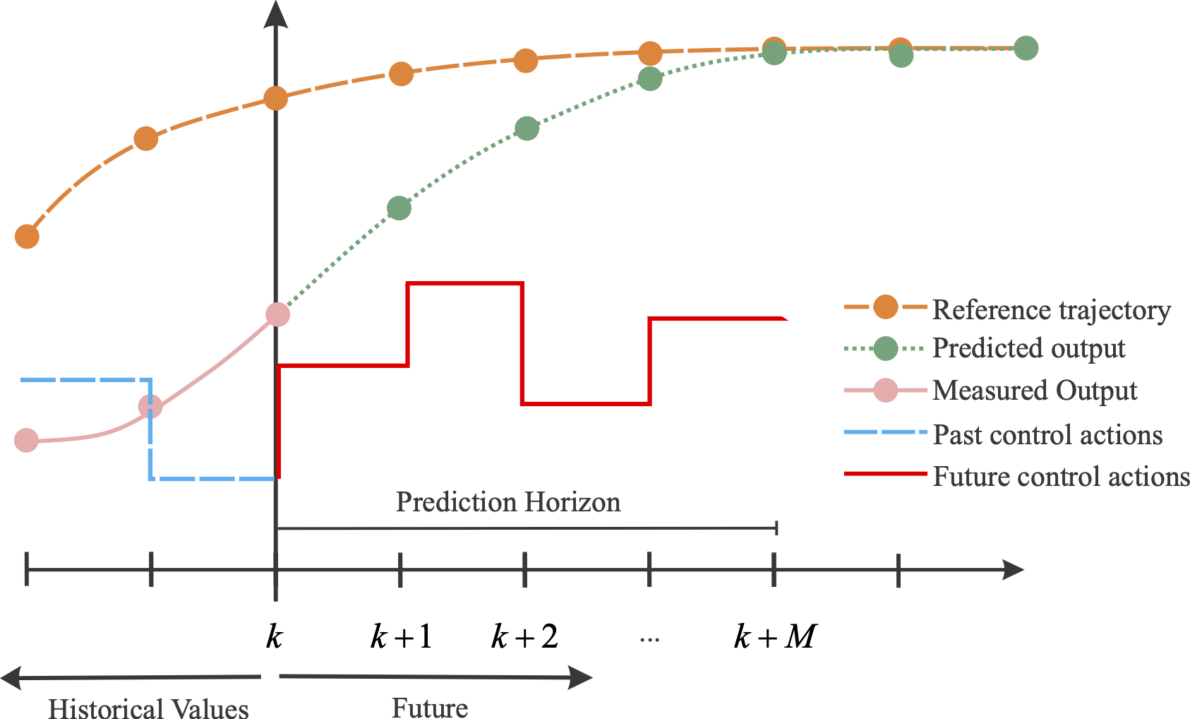
MPC: Representation of the output prediction in a time instant, where the proposed actions generate a predicted behavior that reduces the distance between the value predicted by the model and a reference trajectory:
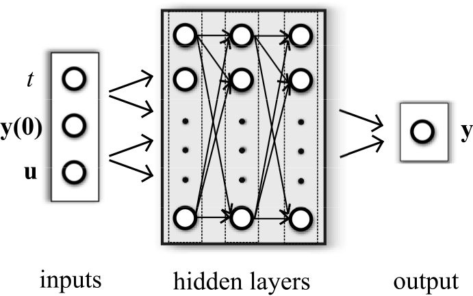
The PINC network has initial state y(0) of the dynamic system and control input u as inputs, in addition to continuous time scalar t. Both y(0) and u can be multidimensional. The output y(t) corresponds to the state of the dynamic system as a function of t 2 [0; T], and initial conditions given by y(0) and u. The deep network is fully connected even though not all connections are shown:
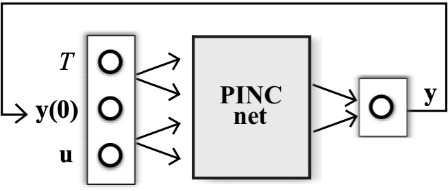
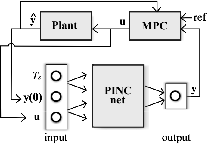
Below, modes of operation of the PINC network. (a) PINC net operates in self-loop mode, using its own output prediction as next initial state, after T seconds. This operation mode is used within one iteration of MPC, for trajectory generation until the prediction horizon of MPC completes (predicted output from the first Figure). (b) Block diagram for PINC connected to the plant. One pass through the diagram arrows corresponds to one MPC iteration applying a control input u for Ts timesteps for both plant and PINC network. Note that the initial state of the PINC net is set to the real output of the plant. In practice, in MPC, these two operation modes are executed in an alternated way (optimization in the prediction horizon, and application of control action).
a).
b)
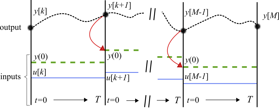
Below, the representation of a trained PINC network evolving through time in self-loop mode (previous Figure a)) for trajectory generation in prediction horizon. The top dashed black curve corresponds to a predicted trajectory y of a hypothetical dynamic system in continuous time. The states y[k] are snapshots of the system in discrete time k positioned at the equidistant vertical lines. Between two vertical lines (during the inner continuous interval between steps k and k + 1), the PINC net learns the solution of an ODE with t \in [0; T], conditioned on a fixed control input u[k] (blue solid line) and initial state y(0) (green thick dashed line). Control action u[k] is changed at the vertical lines and kept fixed for T seconds, and the initial state y(0) in the interval between steps k and k + 1 is updated to the last state of the previous interval k 1 (indicated by the red curved arrow). The PINC net can directly predict the states at the vertical lines without the need to infer intermediate states t < T as numerical simulation does. Here, we assume that T = Ts and, thus, the number of discrete timesteps M is equal to the length of the prediction horizon in MPC.