Physics-informed neural networks (PINNs) impose known physical laws into the learning of deep neural networks, making sure they respect the physics of the process while decreasing the demand of labeled data. For systems represented by Ordinary Differential Equations (ODEs), the conventional PINN has a continuous time input variable and outputs the solution of the corresponding ODE. In their original form, PINNs do not allow control inputs neither can they simulate for long-range intervals without serious degradation in their predictions. In this context, this work presents a new framework called Physics-Informed Neural Nets for Control (PINC), which proposes a novel PINN-based architecture that is amenable to control problems and able to simulate for longer-range time horizons that are not fixed beforehand. The framework has new inputs to account for the initial state of the system and the control action. In PINC, the response over the complete time horizon is split such that each smaller interval constitutes a solution of the ODE conditioned on the fixed values of initial state and control action for that interval. The whole response is formed by feeding back the predictions of the terminal state as the initial state for the next interval. This proposal enables the optimal control of dynamic systems, integrating a priori knowledge from experts and data collected from plants into control applications. We showcase our proposal in the control of two nonlinear dynamic systems: the Van der Pol oscillator and the four-tank system.
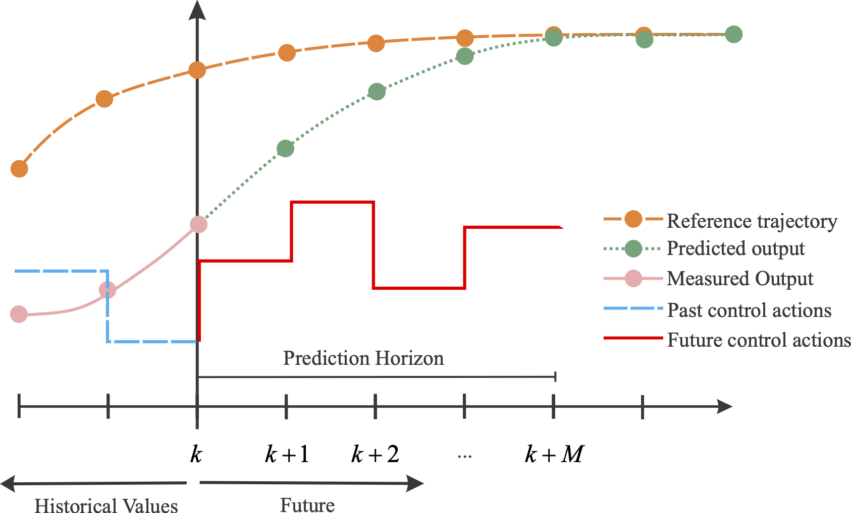
MPC: Representation of the output prediction in a time instant, where the proposed actions generate a predicted behavior that reduces the distance between the value predicted by the model and a reference trajectory:
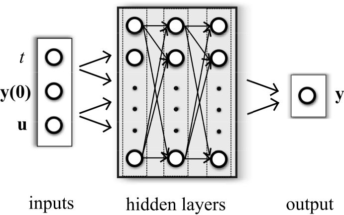
The PINC network has initial state y(0) of the dynamic system and control input u as inputs, in addition to continuous time scalar t. Both y(0) and u can be multidimensional. The output y(t) corresponds to the state of the dynamic system as a function of t 2 [0; T], and initial conditions given by y(0) and u. The deep network is fully connected even though not all connections are shown:
Below, modes of operation of the PINC network. (a) PINC net operates in self-loop mode, using its own output prediction as next initial state, after T seconds. This operation mode is used within one iteration of MPC, for trajectory generation until the prediction horizon of MPC completes (predicted output from the first Figure). (b) Block diagram for PINC connected to the plant. One pass through the diagram arrows corresponds to one MPC iteration applying a control input u for Ts timesteps for both plant and PINC network. Note that the initial state of the PINC net is set to the real output of the plant. In practice, in MPC, these two operation modes are executed in an alternated way (optimization in the prediction horizon, and application of control action).
a). 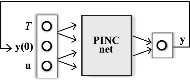
b) 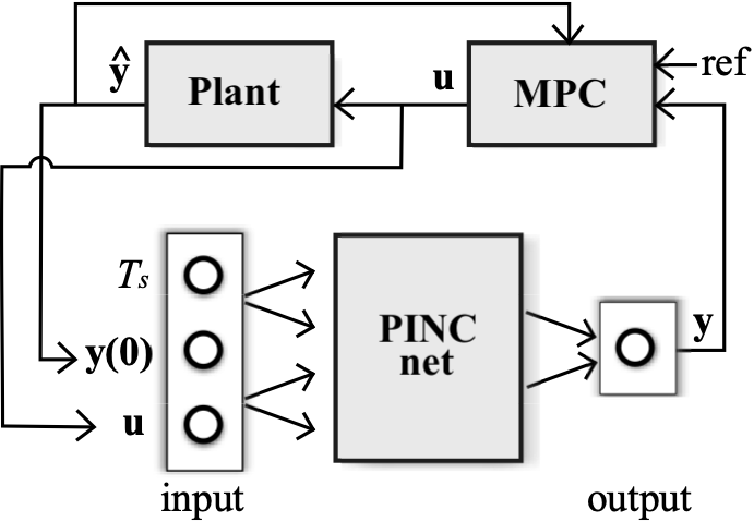
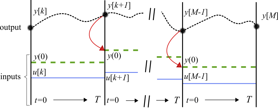
Below, the representation of a trained PINC network evolving through time in self-loop mode (previous Figure a)) for trajectory generation in prediction horizon. The top dashed black curve corresponds to a predicted trajectory y of a hypothetical dynamic system in continuous time. The states y[k] are snapshots of the system in discrete time k positioned at the equidistant vertical lines. Between two vertical lines (during the inner continuous interval between steps k and k + 1), the PINC net learns the solution of an ODE with t \in [0; T], conditioned on a fixed control input u[k] (blue solid line) and initial state y(0) (green thick dashed line). Control action u[k] is changed at the vertical lines and kept fixed for T seconds, and the initial state y(0) in the interval between steps k and k + 1 is updated to the last state of the previous interval k 1 (indicated by the red curved arrow). The PINC net can directly predict the states at the vertical lines without the need to infer intermediate states t < T as numerical simulation does. Here, we assume that T = Ts and, thus, the number of discrete timesteps M is equal to the length of the prediction horizon in MPC.